Brownian motion - with drift
07-Oct-21
A. Fokker-Planck equation
The Fokker-Planck equation is actually the diffusion equation in presence of external potential. It reads
where \(U(x)\) is the external potential, and correspondingly \(F(x)=-U'(x)\) is the external force.
The corresponding Langevin equation to this Fokker-Planck equation reads
Consider the Fokker-Planck equation for linear external potential \(U(x)=-vx\), i.e., constant external force \(F=-U'(x)=v\),
The solution in the infinite domain for the same initial and boundary conditions like for the diffusion equation is the Galilei-shifted Gaussian
B. Simulations
Task2. Simulations explained:
Simulate the Brownian motion with drift, \(v\), by numerical solution of the Langevin equation.
Plot the trajectory and the PDF.
he numerical solution is done by numerical integration of the Langevin equation, i.e.,
Mean squared displacement is given by
Main class for stohastic process:
# Python imports
import seaborn as sns
import matplotlib.pyplot as plt
import numpy as np
import math
from scipy.stats import norm
import warnings
from matplotlib.ticker import (MultipleLocator, AutoMinorLocator)
warnings.filterwarnings("ignore")

# Specifying the figure parameters
font = {'family': 'serif',
        'color': 'black',
        'weight': 'normal',
        'size': 18,
        }
params = {'legend.fontsize': 10,
          'legend.handlelength': 2.}
plt.rcParams.update(params)


# Class for BM stochastic process
class Brownian_motion_Langevin:

    def solve(self):
        """
        Generates all step based the definition for BM, using 2 different approaches.

        Both draw from a Normal Distribution ~ N(0, dt); If dt=1, it is N(0, 1)

        B = B0 + B1*dB1 + ... Bn*dBn = x + v*dt + (2*Dc*dt)^1/2 * N(0, dt)
        :return: None
        """
        # Langevin eq. x(t + 1) = x(t) + v*dt + (2*Dc*dt)^0.5 * normal

        # 1st way - cumulative sum of all noises
        dB = self.initial_y + self.drift * self.delta_t + self.sqrt_2D * self.sqrt_dt * np.random.normal(size=(len(self.times)))
        r1 = np.cumsum(dB)

        # 2nd way - step by step addition
        r2 = np.zeros((len(self.times)))
        for t in range(len(self.times)-1):
            r2[t+1] = r2[t] + self.drift*self.delta_t + self.sqrt_2D * self.sqrt_dt *np.random.normal()

        # Append solutions
        self.numerical_solution = r1
        self.solution = r2

    def __init__(self, drift, diffusion_coefficient, initial_y, simulation_time, sampling_points):
        """

        :param drift: External force - drift
        :param diffusion_coefficient:
        :param initial_y: 1
        :param delta_t: dt - change in time - size of each interval
        :param simulation_time: total time for simulation
        """
        # Initial parameters
        self.drift = drift
        self.diffusion_coefficient = diffusion_coefficient
        self.initial_y = initial_y

        # Define time
        self.simulation_time = simulation_time
        self.sampling_points = sampling_points

        # Get dt
        self.times = np.arange(0,simulation_time+1,1)
        self.delta_t = self.times[1] - self.times[0]

        # Speed up calculations
        self.sqrt_dt = self.delta_t**0.5
        self.sqrt_2D = (2*self.diffusion_coefficient)**0.5

        # Simulate the diffusion process
        self.numerical_solution = []
        self.solution = []
        self.solve()
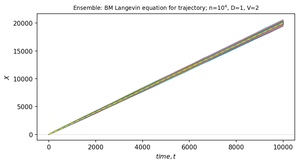
Define start parameters and run/plot ensemble with \(10^4\) processes:
\(n = 10^4\) - Number of simulations
\(V = 2\) - Drift for the diffusion process, v - external force (drift)
\(D = 1\) - Dc - diffusion coefficient
\(dt=1\) - interval size or size step
\(y0 = 0\) - starting point on y axis (theoretical 0 for BM)
\(tt = 10^4\) - total time for each simulation
# Define parametrs for BM process
n = 10_000 # Number of simulations
V = 2  # Drift for the diffusion process, v - external force (drift)
Dc = 1  # Dc - diffusion coefficient
interval_size = 1 # dt = interval_size
y0 = 0  # y0 - starting point
tt = 10_000  # tt - total time for each simulation

# Run simulations
motions = []
for i in range(0, n):
    motions.append(Brownian_motion_Langevin(drift=V,
                                            diffusion_coefficient=Dc,
                                            initial_y=y0,
                                            simulation_time=tt,
                                            sampling_points=interval_size))
# Simple check, how often does the first term (vdt) exceeds the later (2*D*dt)**0.5 * N(0, 1)?
count = 0
for i in range(0, n):
  if (0.5 * interval_size) > ((2 * Dc * interval_size)**0.5 * np.random.normal(scale=interval_size)):
    count += 1

print("The first term exceeds the second: {x:.2f}%".format(x=count/n*100))
The first term exceeds the second: 63.43%
# Plot results
figure, (ax) = plt.subplots(1, 1, figsize=(7, 4), dpi=150)
dist = []
dist2 = []
for i in range(0, n):
    x = motions[i].times
    y1 = motions[i].numerical_solution
    y2 = motions[i].solution

    # Plot way-2
    ax.plot(x, y2, linewidth=1., alpha=0.6, label="BM-drift")

    dist.append(motions[i].numerical_solution)
    dist2.append(motions[i].solution)

plt.axhline(y=0, linewidth=0.5, alpha=0.3, color="black", linestyle='--')

# Plot drift
if V != 0:
    plt.plot(x, V*x, linewidth=.9, alpha=1., color="yellow", linestyle='-.')


plt.ylabel(r"$X$")
plt.xlabel(r"$time, t$")
plt.title(
    r"Ensemble: BM Langevin equation for trajectory; n=$10^4$, D={}, V={}".format(Dc, V),
    fontsize=9)
plt.tight_layout(pad=1.9)
# plt.savefig("Ensemble-beta.png")
plt.show()
# Check shape of lists
print(np.shape(dist2))
print(np.shape(dist))
(10000, 10001)
(10000, 10001)
B.1. Second moment, \(\langle x^2(t) \rangle\)
Mean squared displacement is given by
# Calculations
times = np.arange(0,tt+1,interval_size)
delta_t = times[1] - times[0]
t_frame = times[1]
t = [1, 2, 10]
print("Step size is dt = ", delta_t)

no_simulations, no_points = np.shape(dist)
scale = (no_points/tt)**(1/2)
print("Scale in case of smaler dt, scale={x:.2f}".format(x=scale))

msd = []
msd2 = []

for t in range(no_points-1):
  value_x = [dist[i][t] for i in range(n)]
  value = np.dot(value_x, value_x) / n    # dot product / ensemble size
  msd.append(value)

for t in range(no_points-1):
  value_x = [dist2[i][t] for i in range(n)]
  value = np.dot(value_x, value_x) / n    # dot product / ensemble size
  msd2.append(value)
Step size is dt =  1
Scale in case of smaler dt, scale=1.00
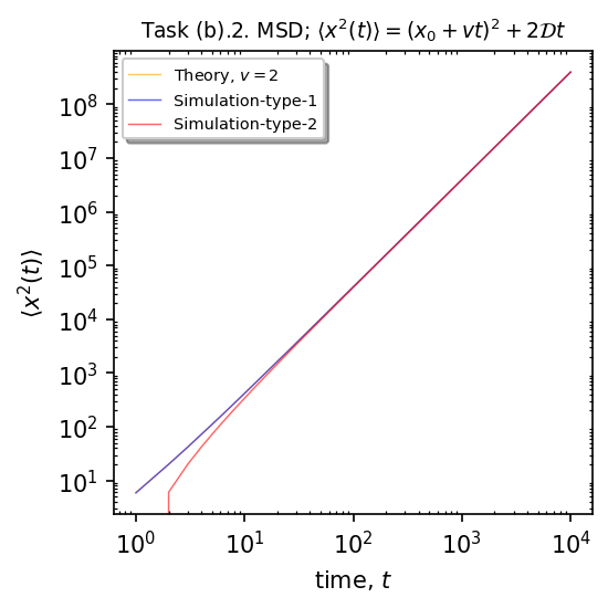
Results
Plot the theoretical (orange) vs the simulation moment (blue-type1, red-type2)
# Theoretical vs. Ensemble
figure, (ax) = plt.subplots(1, 1, figsize=(4, 4), dpi=150)

ax.xaxis.set_minor_locator(AutoMinorLocator())
ax.yaxis.set_minor_locator(AutoMinorLocator())

x = np.arange(1, tt+1, interval_size)
x0 = 0   # x0 in Langevin eq.

ax.plot(x, (lambda x: (x0 + V*x)**2 + 2*Dc*x**1)(x), linewidth=0.7, alpha=0.6, label=r"Theory, $v=${}".format(V), color="orange")
ax.plot(x, msd, 'blue',  markersize=1, linewidth=0.7, alpha=0.6, label=r"Simulation-type-1", markevery=30)
ax.plot(x, msd2, 'red',  markersize=1, linewidth=0.7, alpha=0.6, label=r"Simulation-type-2", markevery=30)

# Add legend if comparing values
plt.legend(loc='upper left',
           fancybox=True,
           shadow=True,
           fontsize='x-small')

ax.set_yscale('log')
ax.set_xscale('log')

plt.ylabel(r"$\langle x^2(t) \rangle$")
plt.xlabel(r"time, $t$")
plt.title(r"Task (b).2. MSD; $\langle x^2(t)\rangle=(x_0 + vt)^2+2\mathcal{D}t$", fontsize=9)
plt.tight_layout(pad=1.9)
ax.tick_params(direction="in", which='minor', length=1.5, top=True, right=True)
# plt.savefig("")
plt.show()
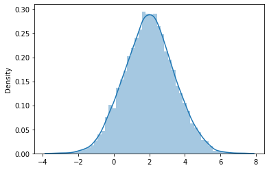
B.2. PDF, \(P(x,t)\)
\(P(x,t)\) is the probability density function (PDF) and \(\mathcal{D}\) is diffusion coefficient, is given by the Gaussian probability density function
We calculate the distributions for 3 different times (\(t=[1, 2, 10]\)) and plot their distribution vs. the theoretical for the exact times
t = [1, 2, 10]
\(t=1\)
# t=1, n=10^4 samples
x_mean_1 = [motions[i].numerical_solution[0] for i in range(0, no_simulations)]

# Print check
print(np.shape(x_mean_1))

mu_1 = np.mean(x_mean_1)

# Print mean, std
print("Mean: ",np.mean(x_mean_1))
print("STD:  ",np.std(x_mean_1))

# Plot dist
x_dots_1 = sns.distplot((scale*np.array(x_mean_1) - mu_1 - y0) + V*t[0]).get_lines()[0].get_data()
(10000,)
Mean:  1.9815428047047756
STD:   1.403877446180871
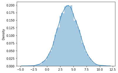
\(t=2\)
# t=2, n=10^4
x_mean_2 = [motions[i].numerical_solution[1] for i in range(0, no_simulations)]

# Print check
print(np.shape(x_mean_2))

mu_2 = np.mean(x_mean_2)

# Print mean, std
print("Mean: ",np.mean(x_mean_2))
print("STD:  ",np.std(x_mean_2))

# Plot dist
x_dots_2 = sns.distplot(scale * np.array(x_mean_2 - mu_2 - y0) + V*t[1]).get_lines()[0].get_data()
(10000,)
Mean:  4.009322812086211
STD:   2.0003013192512364
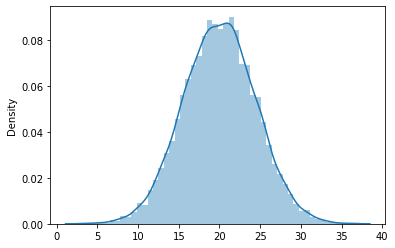
\(t=10\)
# t=3, n=10^4
x_mean_3 = [motions[i].numerical_solution[9] for i in range(0, no_simulations)]
# Print check
print(np.shape(x_mean_3))

mu_3 = np.mean(x_mean_3)
std_3 = np.std(x_mean_3)

# Print mean, std
print("Mean: ",np.mean(x_mean_3))
print("STD:  ",np.std(x_mean_3))

# Plot dist
x_dots_3 = sns.distplot(scale * np.array(x_mean_3 - mu_3 - y0)+V*t[2]).get_lines()[0].get_data()
(10000,)
Mean:  19.993359839345633
STD:   4.428659784044187
Results
# Plot comparison results
from scipy import stats
import seaborn as sns

figure, (ax) = plt.subplots(1, 1, figsize=(7, 4), dpi=200)

x = np.arange(-15,45,0.1)

# Calculate PDF for t=1, t=2 $ t=10
x_0 = 0
t = [1, 2, 10]
f1 = 1/(np.sqrt(4*np.pi*Dc*t[0])) * np.exp(-np.square(x-x_0-V*t[0])/(4*Dc*t[0]))
f2 = 1/(np.sqrt(4*np.pi*Dc*t[1])) * np.exp(-np.square(x-x_0-V*t[1])/(4*Dc*t[1]))
f3 = 1/(np.sqrt(4*np.pi*Dc*t[2])) * np.exp(-np.square(x-x_0-V*t[2])/(4*Dc*t[2]))

# t=1
plt.plot(x_dots_1[0], x_dots_1[1], linewidth=0.6, alpha=0.6, label=r"Ensemble~$t={}$".format(t[0]), color="blue", marker='o',markevery=5, markersize=2)
plt.plot(x, f1, linewidth=0.6, alpha=0.6, label=r"PDF~$t={}$".format(t[0]), color="red")

# t=2
plt.plot(x_dots_2[0], x_dots_2[1], linewidth=0.6, alpha=0.6, label=r"Ensemble~$t={}$".format(t[1]), color="orange", marker='o',markevery=5, markersize=2)
plt.plot(x, f2, linewidth=0.6, alpha=0.6, label=r"PDF~$t={}$".format(t[1]), color="red")

# t=10
plt.plot(x_dots_3[0], x_dots_3[1], linewidth=0.6, alpha=0.6, label=r"Ensemble ~$t={}$".format(t[2]), color="green", marker='o',markevery=5, markersize=2)
plt.plot(x, f3, linewidth=0.6, alpha=0.6, label=r"PDF~$t={}$".format(t[2]), color="red")


# Plot lines for reference
plt.axvline(x=0, linewidth=0.8, alpha=1, color="black")
plt.axvline(x=V, linewidth=0.8, alpha=0.5, color="green", linestyle='--', label=r'$V=${}'.format(V))


# Add legend if comparing values
plt.legend(bbox_to_anchor=(1.05, 1.0),
           loc='upper left',
           fancybox=True,
           shadow=True,
           fontsize='x-small')

plt.ylabel(r"$P(x, t)$")
plt.xlabel(r"$X$")
plt.title(
    r"PDF comparison BM with $V={}$".format(V) + r"; $P(x,t)=\frac{1}{\sqrt{4\pi\mathcal{D}t}}e^{-\frac{(x-x_0-vt)^2}{4\mathcal{D}t}}$",
    fontsize=9, pad=10)
plt.tight_layout(pad=1.9)
ax.tick_params(direction="in", which='minor', length=1.5, top=True, right=True)
# plt.savefig("PDF-Ensemble-t_all-tt_10_v_-1.png")
plt.show()
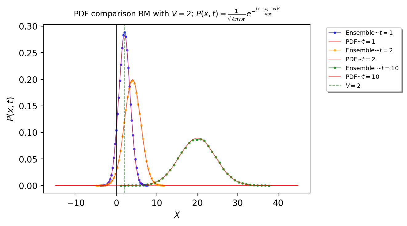
# MSE for each time snapshot
print("t= 1, MSE = {x:.4f}".format(x=np.square(np.subtract(x_dots_1[1], f1[:200])).mean()))
print("t= 2, MSE = {x:.4f}".format(x=np.square(np.subtract(x_dots_2[1], f2[:200])).mean()))
print("t=10, MSE = {x:.4f}".format(x=np.square(np.subtract(x_dots_3[1], f3[:200])).mean()))
t= 1, MSE = 0.0258
t= 2, MSE = 0.0131
t=10, MSE = 0.0017