Backbone explained
A comb model is a particular example of a non-Markovian motion, which takes place due to its specific geometry realization inside a two-dimensional structure. It consists of a backbone along the structure \(x\) axis and fingers along the \(y\) direction, continuously spaced along the \(x\) coordinate, as shown in the figure. This special geometry has been introduced to investigate anomalous diffusion in low-dimensional percolation clusters. In the last decade the comb model has been extensively studied to understand different realizations of non-Markovian random walks, both continuous and discrete. In particular, comb-like models have been used to describe turbulent hyper-diffusion due subdiffusive traps, anomalous diffusion in spiny dendrites, subdiffusion on a fractal comb, and diffusion of light in L’evy glasses as L’evy walks in quenched disordered media, and to model anomalous transport in low-dimensional composites.
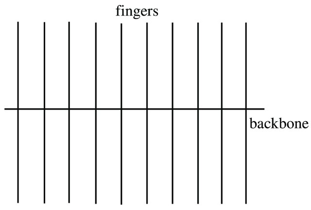
Fig. 1 Comb structure consisting of a backbone and continuously distributed branches/fingers
From the comb structure one can conclude that the diffusion along \(x\)-axis occurs only at \(y=0\) (the backbone), while the diffusion along the \(y\)-axis is normal (Brownian motion). The Brownian particle moving along the backbone can be stuck in the fingers, so there is no movement along the backbone until the particle is returned back to the backbone. Therefore, the fingers play the role of traps. The returning probability of the Brownian particle from the finger to the backbone corresponds to the waiting time PDF for the particle moving along the backbone, so for Brownian motion it scales as \(\sim t^{-3/2}\). From the CTRW theory we know that such waiting times leads to anomalous diffusion with MSD given by \(\langle x^{2}(t)\rangle\sim t^{1/2}\).
The motion along such two-dimensional comb structure can be simulated by the following coupled Langevin equations
where \(\zeta_{i}(t)\) (\(i=\{x,y\}\)) are white Gaussian noise with zero mean \(\langle\zeta_{i}(t)\rangle=0\), and correlation \(\langle\zeta_{i}(t)\zeta_{i}(t')\rangle=\delta(t-t')\), while the function \(A(y)\) is introduced to mimic the motion along the backbone at \(y=0\). As a result, the noise \(\zeta_{x}(t)\) is multiplicative.
To replicate the Dirac \(\delta\)-function, diffusion across the \(x\) direction is permitted in a narrow band of thickness \(2\epsilon\). Another approach is to use \(A(y)=\delta(y)\) and then to employ some approximation formula for the Dirac \(\delta\)-function, for example \(A(y) = \frac{1}{\sqrt{2\pi}\sigma}\exp(-y^2/[2\sigma^2])\) in the limit \(\sigma\to 0\).