Brownian motion - without drift
07-Oct-21
A. Diffusion equation
The solution of the following diffusion equation
in the infinite domain \(x\in(-\infty,\infty)\), for initial condition \(P(x,t=0)=\delta(x-x_0)\) and zero boundary conditions at infinity \(P(x=\pm\infty,t)=0\), where \(P(x,t)\) is the probability density function (PDF) and \(\mathcal{D}\) is diffusion coefficient, is given by the Gaussian probability density function
This diffusion equation describes Brownian motion. The Brownian motion can also be modeled by the Langevin equation
where \(\xi(t)\) is white Gaussian noise with zero mean \(\langle x(t)\rangle=0\) and correlation \(\langle\xi(t)\xi(t')\rangle=\delta(t-t')\).
B. Simulations
Task1. Simulations explained:
Simulate the Brownian motion by numerical solution of the Langevin equation.
Plot the trajectory and the PDF.
The numerical solution is done by numerical integration of the Langevin equation, i.e.,
where \(\zeta(t)\) is a zero-mean Gaussian random variable \(\sim N(0, \Delta t)\).
Mean squared displacement is calculated using
Main class for stohastic process:
# @author: Kiril Zelenkovski

# Python imports
import seaborn as sns
import matplotlib.pyplot as plt
import numpy as np
import math
from scipy.stats import norm
import warnings
from matplotlib.ticker import (MultipleLocator, AutoMinorLocator)
warnings.filterwarnings("ignore")

# Specifying the figure parameters
font = {'family': 'serif',
        'color': 'black',
        'weight': 'normal',
        'size': 18,
        }
params = {'legend.fontsize': 10,
          'legend.handlelength': 2.}
plt.rcParams.update(params)


# Class for BM stochastic process
class Brownian_motion_Langevin:

    def solve(self):
        """
        Generates all step based the definition for BM, using 2 different approaches.

        Both draw from a Normal Distribution ~ N(0, dt); If dt=1, it is N(0, 1)

        B = B0 + B1*dB1 + ... Bn*dBn = x + v*dt + (2*Dc*dt)^1/2 * N(0, dt)
        :return: None
        """
        # Langevin eq. x(t + 1) = x(t) + v*dt + (2*Dc*dt)^0.5 * normal

        # 1st way - cumulative sum of all noises
        dB = self.initial_y + self.drift * self.delta_t + self.sqrt_2D * self.sqrt_dt * np.random.normal(size=(len(self.times)))
        r1 = np.cumsum(dB)

        # 2nd way - step by step addition
        r2 = np.zeros((len(self.times)))
        for t in range(len(self.times)-1):
            r2[t+1] = r2[t] + self.drift*self.delta_t + self.sqrt_2D * self.sqrt_dt *np.random.normal()

        # Append solutions
        self.numerical_solution = r1
        self.solution = r2

    def __init__(self, drift, diffusion_coefficient, initial_y, simulation_time, sampling_points):
        """

        :param drift: External force - drift
        :param diffusion_coefficient:
        :param initial_y: 1
        :param delta_t: dt - change in time - size of each interval
        :param simulation_time: total time for simulation
        """
        # Initial parameters
        self.drift = drift
        self.diffusion_coefficient = diffusion_coefficient
        self.initial_y = initial_y

        # Define time
        self.simulation_time = simulation_time
        self.sampling_points = sampling_points

        # Get dt
        self.times = np.arange(0,simulation_time+1,1)
        self.delta_t = self.times[1] - self.times[0]

        # Speed up calculations
        self.sqrt_dt = self.delta_t**0.5
        self.sqrt_2D = (2*self.diffusion_coefficient)**0.5

        # Simulate the diffusion process
        self.numerical_solution = []
        self.solution = []
        self.solve()
Define start parameters and run/plot ensemble with \(10^4\) processes:
\(n = 10^4\) - Number of simulations
\(V = 0\) - Drift for the diffusion process, v - external force (drift)
\(D = 1\) - Dc - diffusion coefficient
\(dt=1\) - interval size or size step
\(y0 = 0\) - starting point on y axis (theoretical 0 for BM)
\(tt = 10^4\) - total time for each simulation
# Define parametrs for BM process
n = 10_000 # Number of simulations
V = 0  # Drift for the diffusion process, v - external force (drift)
Dc = 1  # Dc - diffusion coefficient
interval_size = 1 # dt = interval_size
y0 = 0  # y0 - starting point
tt = 10_000  # tt - total time for each simulation

# Run simulations
motions = []
for i in range(0, n):
    motions.append(Brownian_motion_Langevin(drift=V,
                                            diffusion_coefficient=Dc,
                                            initial_y=y0,
                                            simulation_time=tt,
                                            sampling_points=interval_size))
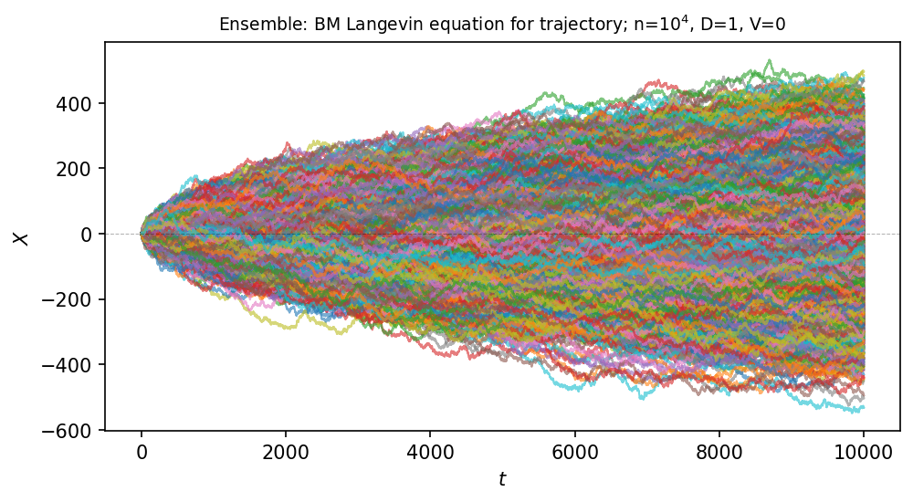
# Plot results from Ensemble
figure, (ax) = plt.subplots(1, 1, figsize=(7, 4), dpi=150)

# Define lists for each solution
dist = []
dist2 = []

for i in range(0, n):
    x = motions[i].times # x- axis (time)
    y1 = motions[i].numerical_solution # Simulation type 1
    y3 = motions[i].solution # Simulation type 2
    ax.plot(x, y3, linewidth=1., alpha=0.6, label="BM-drift")
    dist.append(motions[i].numerical_solution)
    dist2.append(motions[i].solution)

# Add x-axis
plt.axhline(y=0, linewidth=0.5, alpha=0.3, color="black", linestyle='--')

# Add drift function;  if V = 0, no need for plotting it (overlaped with x-axis)
if V != 0:
    plt.plot(x, V*x, linewidth=1., alpha=1., color="yellow", linestyle='-.')

plt.ylabel(r"$X$")
plt.xlabel(r"$t$")
plt.title(
    r"Ensemble: BM Langevin equation for trajectory; n=$10^4$, D={}, V={}".format(Dc, V),
    fontsize=9)
plt.tight_layout(pad=1.9)
# plt.savefig("Ensemble-beta.png")
plt.show()
# Check shape of lists
print(np.shape(dist2))
print(np.shape(dist))
(10000, 10001)
(10000, 10001)
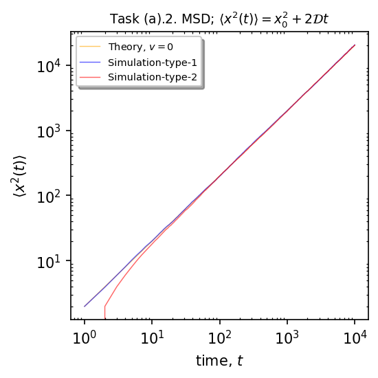
B.1. Second moment, \(\langle x^2(t)\rangle\)
Mean squared displacement is given by
# Calculations
times = np.arange(0,tt+1,interval_size)
delta_t = times[1] - times[0]
t_frame = times[1]
t = [1, 2, 10]
print("Step size is dt = ", delta_t)

no_simulations, no_points = np.shape(dist)
scale = (no_points/tt)**(1/2)
print("Scale in case of smaler dt, scale={x:.2f}".format(x=scale))

msd = []
msd2 = []

for t in range(no_points-1):
  value_x = [dist[i][t] for i in range(n)]
  value = np.dot(value_x, value_x) / n    # dot product / ensemble size
  msd.append(value)

for t in range(no_points-1):
  value_x = [dist2[i][t] for i in range(n)]
  value = np.dot(value_x, value_x) / n    # dot product / ensemble size
  msd2.append(value)
Step size is dt =  1
Scale in case of smaler dt, scale=1.00
Results
Plot the theoretical (orange) vs the simulation moment (blue-type1, red-type2)
# Theoretical vs. Ensemble
figure, (ax) = plt.subplots(1, 1, figsize=(4, 4), dpi=150)

ax.xaxis.set_minor_locator(AutoMinorLocator())
ax.yaxis.set_minor_locator(AutoMinorLocator())

x = np.arange(1, tt+1)
time_t = dt = delta_t
x0 = 0   # mean from PDF

ax.plot(x, (lambda x: (x0 + V*x)**2 + 2*Dc*x**1)(x), linewidth=0.7, alpha=0.6, label=r"Theory, $v=${}".format(V), color="orange")
ax.plot(x, msd, 'blue',  markersize=1, linewidth=0.7, alpha=0.6, label=r"Simulation-type-1", markevery=30)
ax.plot(x, msd2, 'red',  markersize=1, linewidth=0.7, alpha=0.6, label=r"Simulation-type-2", markevery=30)


# Add legend if comparing values
plt.legend(loc='upper left',
           fancybox=True,
           shadow=True,
           fontsize='x-small')

ax.set_yscale('log')
ax.set_xscale('log')

plt.ylabel(r"$\langle x^2(t) \rangle$")
plt.xlabel(r"time, $t$")
plt.title(r"Task (a).2. MSD; $\langle x^2(t)\rangle=x_0^2+2\mathcal{D}t$", fontsize=9)
plt.tight_layout(pad=1.9)
ax.tick_params(direction="in", which='minor', length=1.5, top=True, right=True)
plt.savefig("")
plt.show()
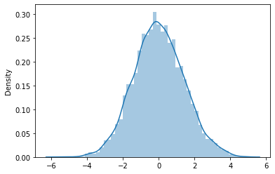
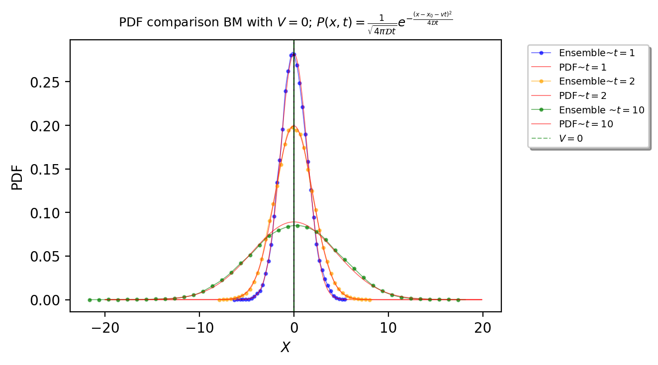
B.2. PDF, \(P(x,t)\)
\(P(x,t)\) is the probability density function (PDF) and \(\mathcal{D}\) is diffusion coefficient, is given by the Gaussian probability density function
We calculate the distributions for 3 different times (\(t=[1, 2, 10]\)) and plot their distribution vs. the theoretical for the exact times
t = [1, 2, 10]
\(t=1\)
# t=1, n=10^4 samples
x_mean_1 = [motions[i].numerical_solution[0] for i in range(0, no_simulations)]
# Print check
print(np.shape(x_mean_1))
mu_1 = np.mean(x_mean_1)
# Print mean, std
print("Mean: ",np.mean(x_mean_1))
print("STD: ",np.std(x_mean_1))
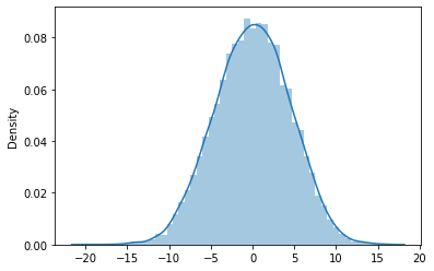
# Plot dist
x_dots_1 = sns.distplot((scale*np.array(x_mean_1) - mu_1 - y0) + V*t[0]).get_lines()[0].get_data()
(10000,)
Mean:  -0.001669172322323002
STD:   1.4132938226483744
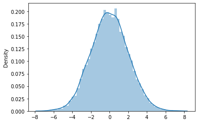
\(t=2\)
# t=2, n=10^4
x_mean_2 = [motions[i].numerical_solution[1] for i in range(0, no_simulations)]

# Print check
print(np.shape(x_mean_2))

mu_2 = np.mean(x_mean_2)

# Print mean, std
print("Mean: ",np.mean(x_mean_2))
print("STD:  ",np.std(x_mean_2))

# Plot dist
x_dots_2 = sns.distplot(scale * np.array(x_mean_2 - mu_2 - y0) + V*t[1]).get_lines()[0].get_data()
(10000,)
Mean:  -0.01599862222285777
STD:   1.9825865412445143
\(t=10\)
# t=3, n=10^4
x_mean_3 = [motions[i].numerical_solution[9] for i in range(0, no_simulations)]
# Print check
print(np.shape(x_mean_3))

mu_3 = np.mean(x_mean_3)

# Print mean, std
print("Mean: ",np.mean(x_mean_3))
print("STD:  ",np.std(x_mean_3))

# Plot dist
x_dots_3 = sns.distplot(scale * np.array(x_mean_3 - mu_3 - y0)+V*t[2]).get_lines()[0].get_data()
(10000,)
Mean:  0.003390582383869105
STD:   4.488405150183261
Results
# Plot comparison results
from scipy import stats
import seaborn as sns

figure, (ax) = plt.subplots(1, 1, figsize=(7, 4), dpi=200)

x = np.arange(-20,20,0.1)

# Calculate PDF for t=1, t=2 $ t=10
x_0 = 0
t = [1, 2, 10]
f1 = 1/(np.sqrt(4*np.pi*Dc*t[0])) * np.exp(-np.square(x-x_0-V*t[0])/(4*Dc*t[0]))
f2 = 1/(np.sqrt(4*np.pi*Dc*t[1])) * np.exp(-np.square(x-x_0-V*t[1])/(4*Dc*t[1]))
f3 = 1/(np.sqrt(4*np.pi*Dc*t[2])) * np.exp(-np.square(x-x_0-V*t[2])/(4*Dc*t[2]))

# t=1
plt.plot(x_dots_1[0], x_dots_1[1], linewidth=0.6, alpha=0.6, label=r"Ensemble~$t={}$".format(t[0]), color="blue", marker='o',markevery=5, markersize=2)
plt.plot(x, f1, linewidth=0.6, alpha=0.6, label=r"PDF~$t={}$".format(t[0]), color="red")

# t=2
plt.plot(x_dots_2[0], x_dots_2[1], linewidth=0.6, alpha=0.6, label=r"Ensemble~$t={}$".format(t[1]), color="orange", marker='o',markevery=5, markersize=2)
plt.plot(x, f2, linewidth=0.6, alpha=0.6, label=r"PDF~$t={}$".format(t[1]), color="red")

# t=10
plt.plot(x_dots_3[0], x_dots_3[1], linewidth=0.6, alpha=0.6, label=r"Ensemble ~$t={}$".format(t[2]), color="green", marker='o',markevery=5, markersize=2)
plt.plot(x, f3, linewidth=0.6, alpha=0.6, label=r"PDF~$t={}$".format(t[2]), color="red")


# Plot lines for reference
plt.axvline(x=0, linewidth=0.8, alpha=1, color="black")
plt.axvline(x=V, linewidth=0.8, alpha=0.5, color="green", linestyle='--', label=r'$V=${}'.format(V))


# Add legend if comparing values
plt.legend(bbox_to_anchor=(1.05, 1.0),
           loc='upper left',
           fancybox=True,
           shadow=True,
           fontsize='x-small')

plt.ylabel("PDF")
plt.xlabel(r"$X$")
plt.title(
    r"PDF comparison BM with $V={}$".format(V) + r"; $P(x,t)=\frac{1}{\sqrt{4\pi\mathcal{D}t}}e^{-\frac{(x-x_0-vt)^2}{4\mathcal{D}t}}$",
    fontsize=9, pad=10)
plt.tight_layout(pad=1.9)
ax.tick_params(direction="in", which='minor', length=1.5, top=True, right=True)
# plt.savefig("PDF-Ensemble-t_all-tt_10_v_-1.png")
plt.show()
# MSE for each time snapshot
print("t= 1, MSE = {x:.4f}".format(x=np.square(np.subtract(x_dots_1[1], f1[:200])).mean()))
print("t= 2, MSE = {x:.4f}".format(x=np.square(np.subtract(x_dots_2[1], f2[:200])).mean()))
print("t=10, MSE = {x:.4f}".format(x=np.square(np.subtract(x_dots_3[1], f3[:200])).mean()))
t= 1, MSE = 0.0212
t= 2, MSE = 0.0120
t=10, MSE = 0.0023